Hall of Fame Model

Table of ContentsClose

1 Activating Python Environment

This code block must be run to activate python virtual environment for org session "SESSION_1". The following Python code blocks are run in "SESSION_1" in which the virtual environment should have been activated.

(pyvenv-activate "~/gitRepos/TTK28-project/venv/")

2 Importing Dependencies

This project is primarily uses Keras and Sklearn for the data analysis itself. For data storage and manipulation pandas and numpy are the primary libraries used. The graphics are generated via matplotlib.

from datetime import datetime
import pandas as pd
import numpy as np
import matplotlib
matplotlib.use('PS')
import matplotlib.pyplot as plt
import logging
from sklearn import tree, decomposition
from sklearn.preprocessing import LabelEncoder
from sklearn.linear_model import LogisticRegression
from sklearn.metrics import confusion_matrix, roc_curve, roc_auc_score, accuracy_score, auc, matthews_corrcoef, make_scorer
from sklearn.utils import class_weight
from sklearn.model_selection import KFold, StratifiedKFold, cross_val_score, cross_validate, learning_curve
from sklearn.pipeline import Pipeline
from sklearn.model_selection import GridSearchCV
import scikitplot as skplt
import tensorflow as tf
from tensorflow import keras
from tensorflow.keras import Model
from tensorflow.keras.callbacks import CSVLogger, ModelCheckpoint
from tensorflow.keras.models import Sequential, model_from_json, load_model
from tensorflow.keras.layers import Dense
from tensorflow.keras.wrappers.scikit_learn import KerasClassifier

3 Hyperparameters

In order to more easily configure the model and keep track of the settting, this hyperparameters dictionary is defined here and used throughout the code where needed.

HP = {
    'NAME': 'full',
    'INFO': 'checking_testing_final',
    'EPOCHS': 50,
    'FOLDS': 2,
    'BATCH_SIZE': 1,
    'OPTIMIZER': 'adam',
    'LOSS': 'binary_crossentropy',
    'METRICS': ['accuracy', 'Recall'],
    'DATASET': 'raw'
}

4 Logging Setup

It was quite hard to keep track of different runs in the project, and noticed I kept loosing track of previous runs and just wanted a log to save some of the metrics and information about the different runs.

4.1 Simply adding whitespace to log file

Nothing special is happening here, but just making sure there is whitespace between runs in the log file.

with open("../result/master_log.txt", "a") as file:
    file.write("\n")
    file.write("\n")
    print(HP, file=file)

4.2 Defining CSVLogger and Tensorboard Settings

CSVLogger is used to keep track of the different runs manually, in addition to setting up tensorboard.

csv_logger = CSVLogger('../result/master_log.txt', append=True, separator=';')
log_dir = "../logs/scalars/" + datetime.now().strftime("%Y%m%d-%H%M%S")
tensorboard_callback = keras.callbacks.TensorBoard(log_dir=log_dir)

4.3 STDOUT Logging Settings

These are the settings for logging information to the terminal and debugging the output.

# logging.basicConfig(encoding='utf-8', level=logging.INFO)

5 Defining Helper Functions

5.1 Creating an ROC Plot

This is a plot that takes in the "false positives" (fper) and "true positives" (tper) and the name of which to save the plot. It generates, shows, and saves an Receiver Operator Characteristics plot which is used for binary classifications problems. A good explanation can be found here.

def plot_roc_curve(fper, tper, name):
    plt.plot(fper, tper, color='orange', label='ROC')
    plt.plot([0, 1], [0, 1], color='darkblue', linestyle='--')
    plt.xlabel('False Positive Rate')
    plt.ylabel('True Positive Rate')
    plt.title('Receiver Operating Characteristic (ROC) Curve')
    plt.legend()
    file_name = '../result/ROC_curve_' + name + datetime.now().strftime("%Y%m%d-%H%M%S") + '.png'
    plt.savefig(file_name)
    plt.savefig("../result/ROC_curve_latest.png")

5.2 Saving and Loading Models

Simply functions to save and load varieties of this hof_model.

def save_model(model, name):
    weights_name = "model_" + name +".h5"
    model.model.save_weights(weights_name)
    print("Saved model to disk")

def load_model(model, name):
    model_name = "model_" + name + ".h5"
    model.load_weights(model_name)
    model.compile(optimizer= HP['OPTIMIZER'], loss= HP['LOSS'], metrics=HP['METRICS'])
    print("Loaded model from disk")
    return model

6 Importing Data

Importing the training and test datasets, in addition to defining the column types to be used of throughout the model.

train_df = pd.read_csv('../data/train_data_' + HP['NAME'] + '.csv', index_col=False)
test_df = pd.read_csv('../data/test_data_' + HP['NAME'] + '.csv', index_col=False)
data_type_dict = {'numerical': [ 'G_all', 'finalGame', 'OPS', 'SB', 'HR', 'Years_Played',
                                 'Most Valuable Player', 'AS_games', 'Gold Glove',
                                 'Rookie of the Year', 'World Series MVP', 'Silver Slugger',
                                 'WHIP', 'ERA', 'KperBB', 'PO', 'A', 'E', 'DP'],
                  'categorical': ['HoF']}

These steps remove the labels from the data sources on both the test and training data.

### Removing the answers for the input data
train_X_raw = train_df.drop(columns=['HoF'])
train_y_raw = train_df['HoF']
test_X_raw = test_df.drop(columns=['HoF'])
test_y_raw = test_df['HoF']

### Converting pandas arrays to numpy arrays
train_X = train_X_raw.to_numpy()
test_X = test_X_raw.to_numpy()

### Creating the label data for the train and test sets
encoder = LabelEncoder()
train_y = encoder.fit_transform(train_y_raw)
test_y = encoder.fit_transform(test_y_raw)

7 Class Weights

One of the ways of dealing with an imbalanced data set is to weight the classes. This suggestion and others are very nicely explained in this post. An error in the one class will have a much higher cost in the cost function. The following backpropagation algorithm will correct the weights based on the ratio between the class weights.

class_weights = class_weight.compute_class_weight('balanced', np.unique(train_y), train_y)
class_weights = dict(enumerate(class_weights))
# class_weights = {0: 1.0, 1: 15.0}
print("class weights: ", class_weights)
print("value counts of Y in train_y: ", train_y.sum())
print("value counts of N in train_y: ", len(train_y) - train_y.sum())

class weights:  {0: 0.5354749704375247, 1: 7.5472222222222225}
value counts of Y in train_y:  180
value counts of N in train_y:  2537

8 Grid Search for Choosing Models

A few different attempts were made to try to compare some different binary classifiers. This is mainly to keep track a backup of notes from the code. There were three different binary classifiers used. Logistic Regression seems to be the standard starting point for binary classification problems. Decisions Trees are flexible, fast, and forgiving so therefore, it was tested as a classifier. The last model was a neural network as it was hoped to be out compete the other classifiers.

Here are some other resources to look through for selection and comparison of different models.

The metric used as the goal for the grid search was the Matthew Correlation Coefficient, which considers an equal weighting of false positive and false negative rates.

8.1 Decision Tree Classifier

pca = decomposition.PCA()
dec_tree = tree.DecisionTreeClassifier()
pipe = Pipeline(steps=[('pca', pca),
                       ('dec_tree', dec_tree)])
n_components = list(range(1,train_X.shape[1]+1,1))
criterion = ['gini', 'entropy']
grid_scorer = make_scorer(matthews_corrcoef, greater_is_better=True)
max_depth = [2,4,6,8,10,12]
parameters = dict(pca__n_components=n_components,
                      dec_tree__criterion=criterion,
                      dec_tree__class_weight=[{0: 1.0, 1: w} for w in [10, 12, 14, 15, 16, 17, 18]],
                      dec_tree__max_depth=max_depth)
clf_GS = GridSearchCV(pipe, parameters, scoring=grid_scorer)
clf_GS.fit(train_X, train_y)
print('Best Score:', clf_GS.best_score_)
print('Best Criterion:', clf_GS.best_estimator_.get_params()['dec_tree__criterion'])
print('Best max_depth:', clf_GS.best_estimator_.get_params()['dec_tree__max_depth'])
print('Best Number Of Components:', clf_GS.best_estimator_.get_params()['pca__n_components'])
print(); print(clf_GS.best_estimator_.get_params()['dec_tree'])

Best Score: 0.5011699881216227
Best Criterion: entropy
Best max_depth: 8
Best Number Of Components: 22

DecisionTreeClassifier(class_weight={0: 1.0, 1: 10}, criterion='entropy',
                       max_depth=8)

8.2 Logistic Regression

logistic_regression = LogisticRegression(random_state=0)
pipe = Pipeline(steps=[('logistic_regression', logistic_regression)])
grid_scorer = make_scorer(matthews_corrcoef, greater_is_better=True)
parameters = dict(logistic_regression__penalty = ['l1', 'l2'],
                  logistic_regression__C = np.logspace(-4, 4, 20),
                  logistic_regression__class_weight=[{0: 1.0, 1: w} for w in [10, 12, 14, 15, 16, 17, 18]],
                  logistic_regression__solver = ['liblinear'])
clf_GS = GridSearchCV(pipe, parameters, scoring=grid_scorer, cv = 5, verbose=True, n_jobs=-1, return_train_score=True)
clf_GS.fit(train_X, train_y)
print('Best Score:', clf_GS.best_score_)
print(); print('Best Estimator:', clf_GS.best_estimator_.get_params()['logistic_regression'])

Fitting 5 folds for each of 280 candidates, totalling 1400 fits
Best Score: 0.6192125559700654

Best Estimator: LogisticRegression(C=29.763514416313132, class_weight={0: 1.0, 1: 10},
                   random_state=0, solver='liblinear')

8.3 Neural Network

Some different model structures were tested for this model, but there were some 'rules of thumb' which were considered. For the number of hidden nodes in a layer:

The number of hidden neurons should be between the size of the input layer and the size of the output layer.
The number of hidden neurons should be 2/3 the size of the input layer, plus the size of the output layer.
The number of hidden neurons should be less than twice the size of the input layer.

A summation of these rules were outlined as the following:

number of hidden layers equals one
the number of neurons in that layer is the mean of the neurons in the input and output layers.

def create_model():
    model = Sequential([
        Dense(26, activation='relu', input_shape=(26,)),
        Dense(17, activation='relu'),
        Dense(9, activation='relu'),
        Dense(1, activation='sigmoid'),
    ])

    model.compile(
        optimizer= HP['OPTIMIZER'],
        loss= HP['LOSS'],
        metrics=HP['METRICS'])
    return model

model = KerasClassifier(build_fn=create_model, verbose = 0)

grid_scorer = make_scorer(matthews_corrcoef, greater_is_better=True)
batch_size = [1, 2, 4]
epochs = [125, 150, 200, 250, 300]
param_grid = dict(batch_size=batch_size,
                  epochs=epochs)
clf_GS = GridSearchCV(model, param_grid, scoring=grid_scorer, cv = 5, n_jobs=-1)
clf_GS.fit(train_X, train_y, class_weight=class_weights)

print('Best Score:', clf_GS.best_score_)
print(); print('Best Estimator:', clf_GS.best_estimator_.get_params())

Best Score: 0.6079706322981303

Best Estimator: {'verbose': 0, 'batch_size': 4, 'epochs': 125, 'build_fn': <function create_model at 0x7fe6b47933a0>}

9 The Final Models

Before each of these models are defined and trained, the checkpointing is set up. These are for setting up the checkpoints while running the model. They are not really in use right now as they are not added in the model.fit callbacks.

9.1 Decision Tree Model

# Checkpointing
model_weights_name = HP['NAME'] + '_decision_tree_model.h5'
checkpointer = ModelCheckpoint(model_weights_name, monitor='Recall', verbose=0)

# Defining and Training the Model
pca = decomposition.PCA(n_components=22)
pca.fit(train_X)
train_X_pca = pca.transform(train_X)
test_X_pca = pca.transform(test_X)

decision_tree_model = tree.DecisionTreeClassifier(criterion='entropy', max_depth=8, class_weight={0: 1.0, 1: 10.0})
decision_tree_model.fit(train_X_pca, train_y)

9.2 Logistic Regression Model

# Checkpointing
model_weights_name = HP['NAME'] + '_logistic_regression_model.h5'
checkpointer = ModelCheckpoint(model_weights_name, monitor='Recall', verbose=0)

# Defining and Training the Model
logistic_regression_model = LogisticRegression(C=29.763514416313132, class_weight={0: 1.0, 1: 10},
                                                random_state=0, solver='liblinear')
logistic_regression_model.fit(train_X, train_y)

9.3 Neural Network Model

# Checkpointing
model_weights_name = HP['NAME'] + '_NN_model.h5'
checkpointer = ModelCheckpoint(model_weights_name, monitor='Recall', verbose=0)

# Defining and Training the Model
def create_model():
    model = Sequential([
        Dense(26, activation='relu', input_shape=(26,)),
        Dense(13, activation='relu'),
        Dense(1, activation='sigmoid'),
    ])

    model.compile(
        optimizer= HP['OPTIMIZER'],
        loss= HP['LOSS'],
        metrics=HP['METRICS'])
    return model

nn_model = KerasClassifier(build_fn=create_model, epochs=HP['EPOCHS'],
                            batch_size=HP['BATCH_SIZE'], verbose = 2)
nn_model.fit(train_X, train_y, class_weight=class_weights, callbacks=[csv_logger, tensorboard_callback])

Epoch 1/50
2717/2717 - 2s - loss: 0.3930 - accuracy: 0.8347 - recall: 0.8111
Epoch 2/50
2717/2717 - 2s - loss: 0.2347 - accuracy: 0.8760 - recall: 0.9056
Epoch 3/50
2717/2717 - 2s - loss: 0.2029 - accuracy: 0.8999 - recall: 0.9500
Epoch 4/50
2717/2717 - 2s - loss: 0.1897 - accuracy: 0.9069 - recall: 0.9333
Epoch 5/50
2717/2717 - 2s - loss: 0.1746 - accuracy: 0.9120 - recall: 0.9444
Epoch 6/50
2717/2717 - 2s - loss: 0.1761 - accuracy: 0.9128 - recall: 0.9444
Epoch 7/50
2717/2717 - 2s - loss: 0.1653 - accuracy: 0.9168 - recall: 0.9500
Epoch 8/50
2717/2717 - 2s - loss: 0.1495 - accuracy: 0.9257 - recall: 0.9611
Epoch 9/50
2717/2717 - 2s - loss: 0.1433 - accuracy: 0.9201 - recall: 0.9667
Epoch 10/50
2717/2717 - 2s - loss: 0.1492 - accuracy: 0.9293 - recall: 0.9500
Epoch 11/50
2717/2717 - 2s - loss: 0.1391 - accuracy: 0.9249 - recall: 0.9611
Epoch 12/50
2717/2717 - 2s - loss: 0.1238 - accuracy: 0.9371 - recall: 0.9778
Epoch 13/50
2717/2717 - 2s - loss: 0.1243 - accuracy: 0.9356 - recall: 0.9722
Epoch 14/50
2717/2717 - 2s - loss: 0.1405 - accuracy: 0.9360 - recall: 0.9444
Epoch 15/50
2717/2717 - 2s - loss: 0.1133 - accuracy: 0.9400 - recall: 0.9833
Epoch 16/50
2717/2717 - 2s - loss: 0.1081 - accuracy: 0.9455 - recall: 0.9667
Epoch 17/50
2717/2717 - 2s - loss: 0.1063 - accuracy: 0.9488 - recall: 0.9778
Epoch 18/50
2717/2717 - 2s - loss: 0.1094 - accuracy: 0.9411 - recall: 0.9722
Epoch 19/50
2717/2717 - 2s - loss: 0.0986 - accuracy: 0.9544 - recall: 0.9778
Epoch 20/50
2717/2717 - 2s - loss: 0.0985 - accuracy: 0.9525 - recall: 0.9778
Epoch 21/50
2717/2717 - 2s - loss: 0.0986 - accuracy: 0.9514 - recall: 0.9889
Epoch 22/50
2717/2717 - 2s - loss: 0.1130 - accuracy: 0.9499 - recall: 0.9778
Epoch 23/50
2717/2717 - 2s - loss: 0.0900 - accuracy: 0.9551 - recall: 0.9833
Epoch 24/50
2717/2717 - 2s - loss: 0.0887 - accuracy: 0.9584 - recall: 0.9667
Epoch 25/50
2717/2717 - 2s - loss: 0.0826 - accuracy: 0.9591 - recall: 0.9944
Epoch 26/50
2717/2717 - 2s - loss: 0.0994 - accuracy: 0.9577 - recall: 0.9889
Epoch 27/50
2717/2717 - 2s - loss: 0.0834 - accuracy: 0.9614 - recall: 0.9833
Epoch 28/50
2717/2717 - 2s - loss: 0.0790 - accuracy: 0.9647 - recall: 0.9889
Epoch 29/50
2717/2717 - 2s - loss: 0.0790 - accuracy: 0.9658 - recall: 0.9778
Epoch 30/50
2717/2717 - 2s - loss: 0.0794 - accuracy: 0.9639 - recall: 0.9889
Epoch 31/50
2717/2717 - 2s - loss: 0.0789 - accuracy: 0.9625 - recall: 0.9833
Epoch 32/50
2717/2717 - 2s - loss: 0.0795 - accuracy: 0.9610 - recall: 0.9833
Epoch 33/50
2717/2717 - 2s - loss: 0.0918 - accuracy: 0.9628 - recall: 0.9833
Epoch 34/50
2717/2717 - 2s - loss: 0.0811 - accuracy: 0.9632 - recall: 0.9833
Epoch 35/50
2717/2717 - 2s - loss: 0.0827 - accuracy: 0.9606 - recall: 0.9722
Epoch 36/50
2717/2717 - 2s - loss: 0.0796 - accuracy: 0.9614 - recall: 0.9889
Epoch 37/50
2717/2717 - 2s - loss: 0.0662 - accuracy: 0.9680 - recall: 0.9833
Epoch 38/50
2717/2717 - 2s - loss: 0.0686 - accuracy: 0.9654 - recall: 0.9889
Epoch 39/50
2717/2717 - 2s - loss: 0.0632 - accuracy: 0.9661 - recall: 0.9944
Epoch 40/50
2717/2717 - 2s - loss: 0.0696 - accuracy: 0.9661 - recall: 0.9833
Epoch 41/50
2717/2717 - 2s - loss: 0.0661 - accuracy: 0.9739 - recall: 0.9944
Epoch 42/50
2717/2717 - 2s - loss: 0.0682 - accuracy: 0.9672 - recall: 0.9833
Epoch 43/50
2717/2717 - 2s - loss: 0.0592 - accuracy: 0.9731 - recall: 0.9833
Epoch 44/50
2717/2717 - 2s - loss: 0.0539 - accuracy: 0.9772 - recall: 0.9944
Epoch 45/50
2717/2717 - 2s - loss: 0.0727 - accuracy: 0.9750 - recall: 0.9889
Epoch 46/50
2717/2717 - 2s - loss: 0.0587 - accuracy: 0.9750 - recall: 0.9944
Epoch 47/50
2717/2717 - 2s - loss: 0.0584 - accuracy: 0.9709 - recall: 1.0000
Epoch 48/50
2717/2717 - 2s - loss: 0.0602 - accuracy: 0.9757 - recall: 0.9833
Epoch 49/50
2717/2717 - 2s - loss: 0.0550 - accuracy: 0.9728 - recall: 0.9889
Epoch 50/50
2717/2717 - 2s - loss: 0.0742 - accuracy: 0.9713 - recall: 0.9889

10 Generating Predictions and Prediction Probabilities

The model.predict() will return the class predictions for the input data put in the function. The model.predict_proba() will return the probability predictions for the classes, and is the likelihood of the observation belonging to the different classes.

# Testing the Decision Tree Model
decision_tree_pred = decision_tree_model.predict(test_X_pca)
decision_tree_y_score = decision_tree_model.predict_proba(test_X_pca)
# Testing the Logistic Regression Model
logistic_regression_pred = logistic_regression_model.predict(test_X)
logistic_regression_y_score = logistic_regression_model.predict_proba(test_X)
# Testing the Neural Network Model
nn_pred = nn_model.predict(test_X)
nn_y_score = nn_model.predict_proba(test_X, batch_size=HP['BATCH_SIZE'])

11 Metrics

Since the data set is imbalanced, there are other metrics to consider beyond the typical accuracy. In this dataset the ratio of HoF players vs. non-HoF players is 14:1 after preprocessing. Without class weights there could be a bias towards never selecting the HoF players resulting an accuracy over 90% while always predicting them as non-HoF players.

# Calculating overall metrics
def print_metrics(test_y, pred, y_score, model_name):
    accuracy = accuracy_score(test_y, pred)
    mcc = matthews_corrcoef(test_y, pred)
    tn, fp, fn, tp = confusion_matrix(test_y, pred).ravel()
    confusion_mat = [tn, fp, fn, tp]
    auroc = roc_auc_score(test_y, y_score[:,0])
    precision = tp/(tp+fp)
    recall = tp/(tp+fn)
    f1 = (2*precision*recall)/(precision+recall)

    # Showing numerical results
    confusion_label = ["tn", "fp", "fn", "tp"]
    for i in range(0,len(confusion_mat)):
        print(confusion_label[i], ': ', confusion_mat[i])
    print("###### ---------Overall Results --------- ######")
    print("model_name: ", model_name)
    print("accuracy: ", accuracy)
    print("MCC: ", mcc)
    print("confusion_mat: ", confusion_mat)
    print("auroc: ", auroc)
    print("precision: ", precision)
    print("recall: ", recall)
    print("f1: ", f1)
    print("")

    # Saving the metrics
    metric_dict = {
        'Model Name': model_name,
        'True Negative': tn,
        'True Positive': tp,
        'False Negative': fn,
        'False Positive': fp,
        'AUROC': auroc,
        'Accuracy': accuracy,
        'Precision': precision,
        'Recall': recall,
        'F1': f1
    }
    with open("../result/master_log.txt", "a") as file:
        print(metric_dict, file=file)

print_metrics(test_y, decision_tree_pred, decision_tree_y_score, "Decision Tree")
print_metrics(test_y, logistic_regression_pred, logistic_regression_y_score, "Logistic Regression")
print_metrics(test_y, nn_pred, nn_y_score, "Neural Network")

tn :  576
fp :  58
fn :  22
tp :  23
###### ---------Overall Results --------- ######
model_name:  Decision Tree
accuracy:  0.882179675994109
MCC:  0.3220495679851962
confusion_mat:  [576, 58, 22, 23]
auroc:  0.2860848229933403
precision:  0.2839506172839506
recall:  0.5111111111111111
f1:  0.3650793650793651

tn :  572
fp :  62
fn :  8
tp :  37
###### ---------Overall Results --------- ######
model_name:  Logistic Regression
accuracy:  0.8969072164948454
MCC:  0.5106413422190602
confusion_mat:  [572, 62, 8, 37]
auroc:  0.05341745531019977
precision:  0.37373737373737376
recall:  0.8222222222222222
f1:  0.513888888888889

tn :  596
fp :  38
fn :  15
tp :  30
###### ---------Overall Results --------- ######
model_name:  Neural Network
accuracy:  0.9219440353460973
MCC:  0.502772043165843
confusion_mat:  [596, 38, 15, 30]
auroc:  0.07173151069050122
precision:  0.4411764705882353
recall:  0.6666666666666666
f1:  0.5309734513274336

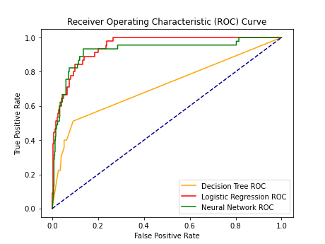
12 Plots

Three metrics that are smart to include for imbalanced datasets are:

ROC curve
Confusion Matrix
Precision-Recall Matrix

# ROC curve
decision_tree_fper, decision_tree_tper, thresholds = roc_curve(test_y, decision_tree_y_score[:,1])
logistic_regression_fper, logistic_regression_tper, thresholds = roc_curve(test_y, logistic_regression_y_score[:,1])
nn_fper, nn_tper, thresholds = roc_curve(test_y, nn_y_score[:,1])

plt.plot(decision_tree_fper, decision_tree_tper, color='orange', label='Decision Tree ROC')
plt.plot(logistic_regression_fper, logistic_regression_tper, color='red', label='Logistic Regression ROC')
plt.plot(nn_fper, nn_tper, color='green', label='Neural Network ROC')
plt.plot([0, 1], [0, 1], color='darkblue', linestyle='--')
plt.xlabel('False Positive Rate')
plt.ylabel('True Positive Rate')
plt.title('Receiver Operating Characteristic (ROC) Curve')
plt.legend()
file_name = '../result/ROC_curve_' + HP['NAME'] + datetime.now().strftime("%Y%m%d-%H%M%S") + '.png'
plt.savefig(file_name)
plt.savefig("../result/ROC_curve_latest.png")
plt.clf()

decision_tree_man_auroc = auc(decision_tree_fper, decision_tree_tper)
logistic_regression_man_auroc = auc(logistic_regression_fper, logistic_regression_tper)
nn_man_auroc = auc(nn_fper, nn_tper)
print("decision_tree_man_auroc: ", decision_tree_man_auroc)
print("logistic_regression_man_auroc: ", logistic_regression_man_auroc)
print("nn_man_auroc: ", nn_man_auroc)

decision_tree_man_auroc:  0.7139151770066596
logistic_regression_man_auroc:  0.9465825446898002
nn_man_auroc:  0.9232211706975114

The latest ROC_plot is the following plot.

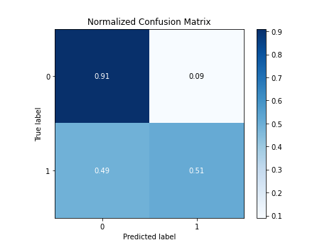
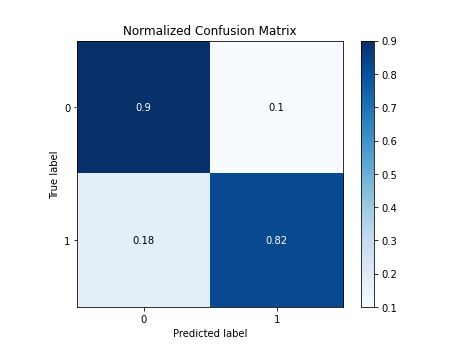
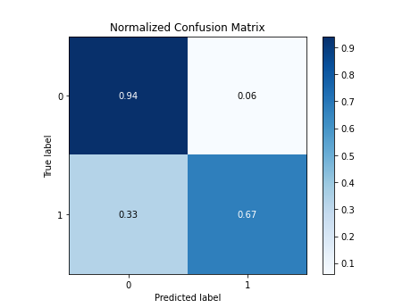
# Generating a confusion matrix
def create_confusion_matrix(test_y, pred, model_name):
    skplt.metrics.plot_confusion_matrix(test_y, pred, normalize=True)
    confusion_mat_string = "../result/confusion_mat_" + HP['NAME'] + model_name + datetime.now().strftime("%Y%m%d-%H%M%S") + ".png"
    plt.savefig(confusion_mat_string)
    latest_model_name = "../result/confusion_mat_" + model_name + "_latest.png"
    plt.savefig(latest_model_name)
    plt.clf()

create_confusion_matrix(test_y, decision_tree_pred, "decision_tree")
create_confusion_matrix(test_y, logistic_regression_pred, "logistic_regression")
create_confusion_matrix(test_y, nn_pred, "nn")

Confusion Matrix for the Decision Tree Classifier

Confusion Matrix for the Logistic Regression Classifier

Confusion Matrix for the Neural Network Model

# Generating precision-recall curve
def create_precision_recall_curve(test_y, y_score, model_name):
    skplt.metrics.plot_precision_recall(test_y, y_score)
    precision_recall_curve_string = "../result/precision_recall_curve_" + HP['NAME'] + "_" + model_name + "_" + datetime.now().strftime("%Y%m%d-%H%M%S") + ".png"
    plt.savefig(precision_recall_curve_string)
    latest_name = "../result/precision_recall_curve_" + model_name + "_latest.png" 
    plt.savefig(latest_name)
    plt.clf()

create_precision_recall_curve(test_y, decision_tree_y_score, "decision_tree")
create_precision_recall_curve(test_y, logistic_regression_y_score, "logistic_regression")
create_precision_recall_curve(test_y, nn_y_score, "nn")

Precision-Recall Curve for the Decision Tree Classifier

Precision-Recall Curve for the Logistic Regression

Precision-Recall Curve for the Neural Network

13 Links to Other Files in Project

extract_data: Extracting data from Lahman's raw data.
filter_data: Data manipulation, feature creation and feature selection.
hof_model: Creation of the model and training of the neural network.
grid_search_results: Storing some of the results for the best Grid Searches